Building an Anomaly Detection System with Recurrent Neural Networks
Introduction
Industrial plants, aircraft, cybersecurity, but also medicine, finance, and more: anomaly detection systems serve a vital role in numerous contexts, promptly identifying malfunctions and irregularities without the need for (and often outperforming) constant expert oversight. There are multiple types of anomaly detection. In this article, I will demonstrate how to use neural networks to build a simple anomaly detection system specifically for time series data, i.e., the kind of data that is mostly generated by sensors.
The only prerequisites are average programming skills, but some basic understanding of machine learning can be helpful too. A Google Colab notebook with the code for this article is also available.
What is an anomaly?
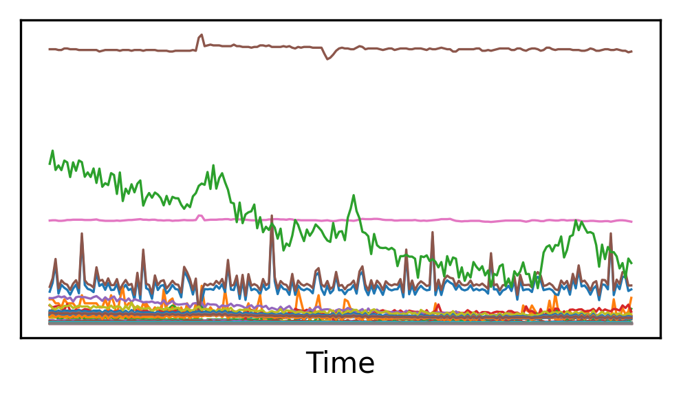
Within a system, an anomaly is a deviation from the expected behavior. Take a look at the pictures below:
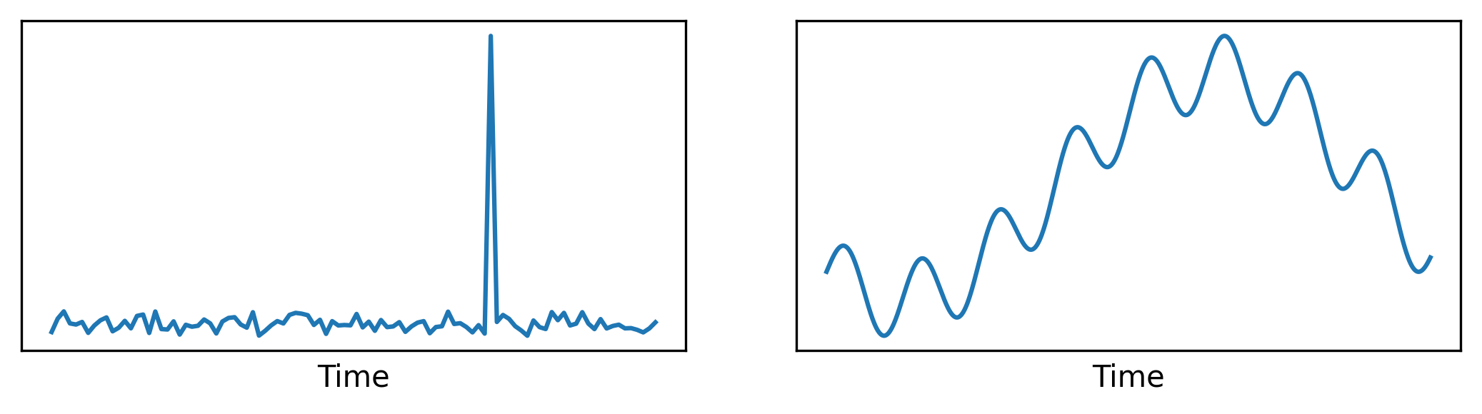
Even without knowing anything about the source of this data, you would likely tell that the spike on the left plot is probably an anomaly. Intuitively, we imagine tracing a horizontal line over that graph: anything above that, it is an anomaly. With the plot on the right though, it’s not that simple. Is there an anomaly? And if so, what’s the rule to identify it? Is there a rule at all?
To determine whether the plot on the right is showing an anomaly, we would have to compare it with an example of known normal behavior for the same data source. We can’t just use a threshold: perhaps the values are supposed to grow and shrink, but when they stop moving, that could be the actual anomaly. To make this even more complex, in real world scenarios one often doesn’t have access to examples of anomalies, or the number of examples that one can get is insufficient for any meaningful use.
How can we, then, identify an anomaly without knowing how an anomaly looks like? In the rest of this article, I am going to show how we can use a neural network to encode the normal behavior of a time series, and then detect deviations from it, assuming no knowledge at all of what anomalies may look like.
Detecting anomalies
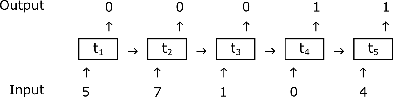
Recurrent Neural Networks (RNNs)1 are machine learning models that can be trained to perform predictions on temporal data. Typically, RNNs accept a sequence as input, and produce another sequence as output. In our case, the task could be for the network to classify, for each time step of the input sequence, whether it represents an anomaly. The output would then be a sequence of ones (corresponding to anomalous time steps) and zeros, just like I show in the picture below. As I anticipated, though, labeled anomalous data is likely to be non-existent, since anomalies are often rare. This makes it impossible to apply a supervised end-to-end learning method that trains the network to classify anomalies by exhibiting examples of those.
With the assumption that we only have access to unlabeled examples of normal behavior, we can do something else. We can train the network to learn a representation of normal behavior, so that we can detect when the actual behavior deviates from it. In fact, a typical method for modeling the behavior of a system is what is called next step prediction: the network is trained to predict the next step that will come in a sequence of data points.
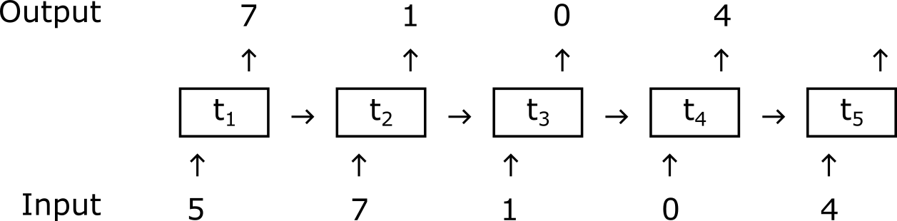
After the network has been trained to do next step prediction, we can feed it live data and the network will try to anticipate what will come next. We can then compare the network prediction at time \(t\), which we call \(y_{t}\), with the actual value of the next step \(x_{t+1}\). If the network was trained successfully, \(y_{t}\) and \(x_{t+1}\) will often be similar. But if the next step \(x_{t+1}\) is anomalous, the network could fail to predict it correctly: in that case, we may expect a significant discrepancy between \(y_{t}\) and \(x_{t+1}\).
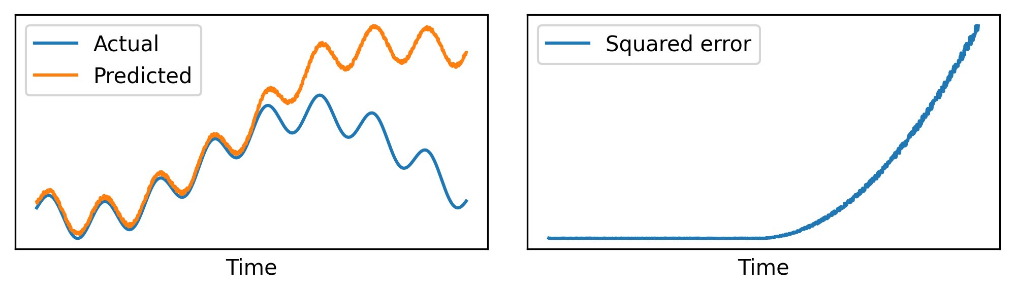
As shown in the figure above, we now have a way to detect anomalies: when the prediction error between \(y_{t}\) and \(x_{t+1}\) is greater than a given threshold (which we will see how to compute), we mark it as an anomaly. For now, we only considered scalar signals: in that case, to compute the prediction error we can simply take the difference \((y_{t} - x_{t+1})\), and then square it to always get a non-negative number* to obtain \((y_{t} - x_{t+1})^2\). In general, though, our signals might be composed by multiple features or components. To support that, we use the Mean Squared Error (MSE), which is just a generalization of the previous formula over vectors: it takes two n-dimensional vectors as input, and returns a single scalar value (the mean squared error) as output.
Network Architecture
Instead of a vanilla RNN, which notoriously exhibits difficulties when trained by backpropagation2, we are going to use a variant named Gated Recurrent Unit (GRU)3.
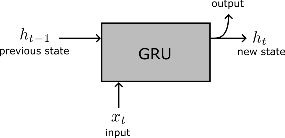
For the purposes of this article, you don’t have to know the details of how a GRU works. All you need is to understand the picture above: a GRU takes two inputs (its own state at the previous time step, \(h_{t-1}\) and the data input at the current time step, \(x_t\)), and outputs a new state \(h_t\) that will be fed back to itself at the next time step. The output state can also be used as the “data output” of the GRU (but, really, it is the same).
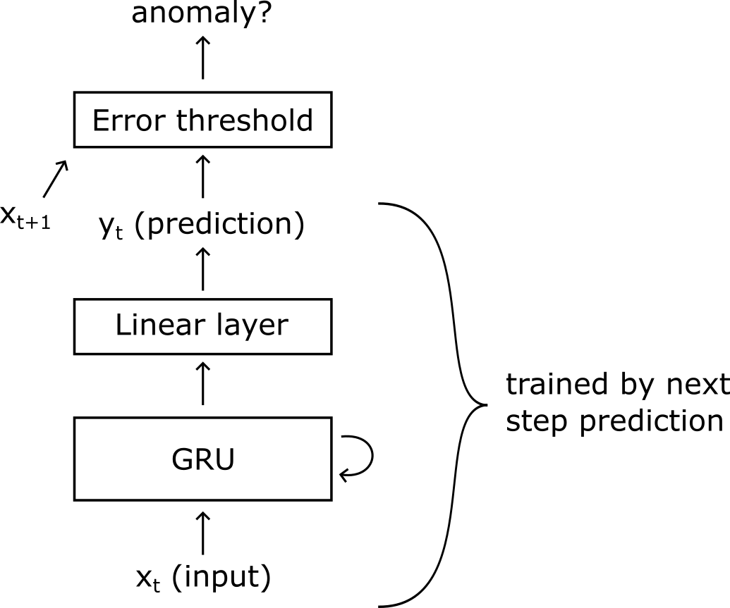
In the picture above, I illustrate the architecture of the system. First, the input sequence \(\mathbf{x} = [x_1, x_2, …, x_t]\) is fed to the GRU, together with the output of the GRU at the previous time step. At each time step, the output of the GRU is then consumed by a linear neural layer, which emits a prediction. One of the reasons why the linear layer is there, is to decouple the size of the hidden state \(h_t\) with the size of the output, so that we can decide the size of the network independently of the input and output sizes. The GRU and the linear layer are jointly trained to predict the next step of the input sequence.
After a prediction \(y_t\) is obtained, we observe the input at the next time step \(x_{t+1}\) and we compute the prediction error, which is then compared to a threshold to determine if \(x_{t+1}\) is an anomaly.
Computation of the threshold
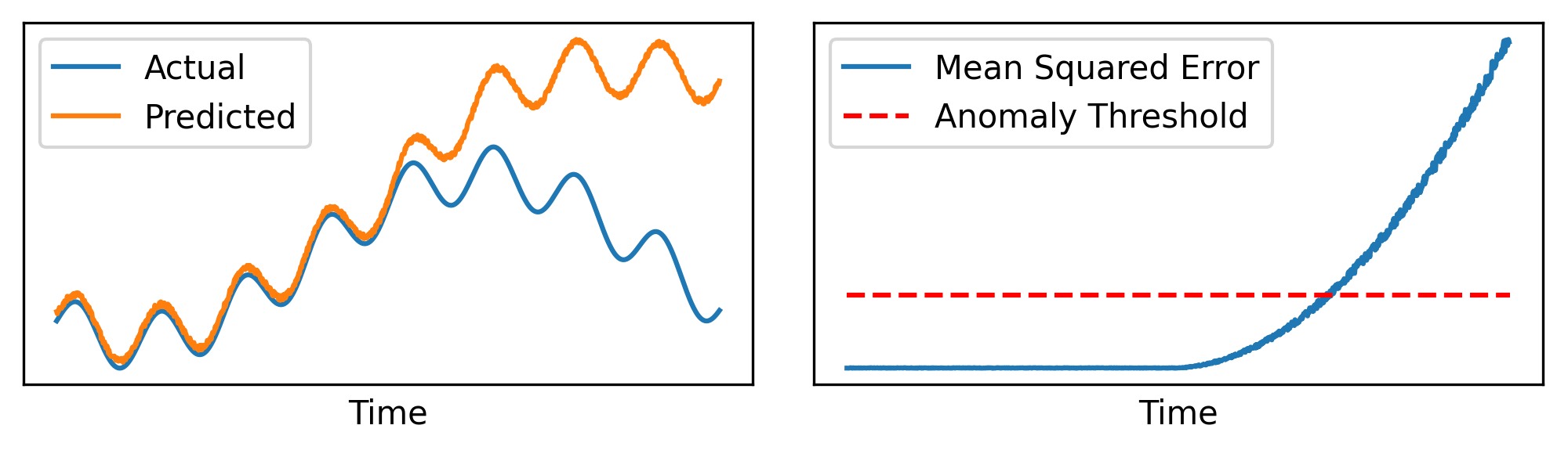
How much of an error is “too much”? We would like to establish a threshold value at which, when the prediction error surpasses it, we can confidently identify it as an anomaly (see the figure below).
We can expect the value of the ideal error threshold to vary depending on various factors, such as the difficulty of the problem. Moreover, since we don’t have labeled data, we cannot really fine-tune the threshold to the optimal value. While there are advanced techniques that allow computing dynamic thresholds4, for simplicity we can opt for the following threshold \(\epsilon\), which allows for some basic level of automatic adaptation with respect to the data. Assume \(\mathbf{e} = [\text{MSE}(y_1, x_{2}), \dots, \text{MSE}(y_t, x_{t+1})]\) is the vector containing all the mean squared errors for each time step (or, at least, a window of time steps). We can compute:
\[ \epsilon = \mu(\mathbf{e}) + z \sigma(\mathbf{e}), \]
where \(\mu(\mathbf{e})\) and \(\sigma(\mathbf{e})\) are respectively the mean and the standard deviation of \(\mathbf{e}\), and \(z\) is a constant that determines the sensitivity of the detection. We are going to use \(z=5\), but in practice this is a value that can be manually tuned, even after the model has been deployed.
While not very advanced, this method gives us a reasonable enough baseline to demonstrate the concept.
The Dataset
To test our algorithm, we are going to use the Server Machine Dataset5. This dataset contains data for 12 machines, and for each machine there are 38 metrics that have been measured at 60 seconds intervals. For simplicity, we are going to use the pre-processed SMD dataset from InterFusion6.
To make training easier, we normalize the data so that all the 38 features vary in roughly the same range when going in and coming out of the neural network. To do this, we compute the max and min of each feature in the training set, and then we rescale it a range between \(0\) and \(1\):
\[x’ = (x - x_{min}) / (x_{max} - x_{min}).\]
After training, we reuse the original max and min to also rescale the test data.
Finally, for each machine, the dataset already provides a training/test split. We will use the test set (which does contain labeled anomalies) only for assessing the predictive performance of our algorithm. In addition, we extract the last 20% of the training set to serve as a validation set, to select the best model among different configurations of the hyperparameters.
Writing the code
The code is written in Python, using the popular PyTorch library. I also prepared a Google Colab notebook: I strongly suggest following along on that notebook to fully understand how the code works (you get to try it on a GPU too). I will not include the full code in this post, just some highlights of the most interesting parts.
If you’d like to skip the code for now, you can jump straight to the Results section, where I show some examples of our model in action.
Datasets
To facilitate training, we start by splitting the training set into a set of sequences of length 60 each. We then associate each sequence with a target vector, which represents the next time step after the end of the sequence (what we need to predict). Finally, we normalize the data. We wrap all this into a class that we call MachineTrainDataset:
class MachineTrainDataset(torch.utils.data.Dataset):
    def __init__(self, machine_name):
        """
        :param machine_name  the name of the machine from the dataset, e.g. "machine-1-1"
        """
        with open(os.path.join(ds_path, f"{machine_name}_train.pkl"), 'rb') as f:
            self.train = torch.from_numpy(pickle.load(f)).to(device)
        self.seq_len = 60
        self.num_seqs = len(self.train) - self.seq_len

        # Normalization
        span = self.train.max(dim=0)[0] - self.train.min(dim=0)[0]
        span[span==0] = 1
        self.train = (self.train - self.train.min(dim=0)[0]) / span

    def __len__(self):
        return self.num_seqs

    def __getitem__(self, idx):
        """
        Returns:
         - an input vector of shape (seq_len, n_feats)
         - a target vector of shape (n_feats)
        """
        return self.train[idx:idx+self.seq_len], self.train[idx+self.seq_len]
For the test dataset, we don’t split the data into multiple sequences. Instead, we return each time step separately, paired with its label (1 if it is an anomaly, 0 otherwise). We also perform normalization, but we use the max and min values from the training set, to ensure the test data is scaled uniformly with the data used for training. We call this the MachineTestDataset:
class MachineTestDataset(torch.utils.data.Dataset):
    def __init__(self, machine_name):
        """
        :param machine_name  the name of the machine from the dataset, e.g. "machine-1-1"
        """
        with open(os.path.join(ds_path, f"{machine_name}_test.pkl"), 'rb') as f:
            train = torch.from_numpy(pickle.load(f)).to(device)
        with open(os.path.join(ds_path, f"{machine_name}_test.pkl"), 'rb') as f:
            self.test = torch.from_numpy(pickle.load(f)).to(device)
        with open(os.path.join(ds_path, f"{machine_name}_test_label.pkl"), 'rb') as f:
            self.test_label = torch.from_numpy(pickle.load(f)).to(device=device, dtype=int)
        assert len(self.test) == len(self.test_label)

        # Normalization (with respect to the training data)
        span = train.max(dim=0)[0] - train.min(dim=0)[0]
        span[span==0] = 1
        self.test = (self.test - train.min(dim=0)[0]) / span

    def __len__(self):
        return len(self.test)

    def __getitem__(self, idx):
        return self.test[idx], int(self.test_label[idx])
The model
Our machine learning model is as simple as it can be. A GRU with input size \(n_x = 38\) processes the input sequence one step at a time, producing a hidden state of size \(n_h\). Then, the hidden state is fed to a linear layer which tries to predict the next input. We call this the AnomalyDetector:
class AnomalyDetector(nn.Module):
    def __init__(self, n_x, n_h):
        """
        :param n_x  the number of features in the input
        :param n_h  the size of the hidden state of the recurrent network
        """
        super().__init__()
        self.rnn = nn.GRU(n_x, n_h)
        self.out = nn.Linear(n_h, n_x)

    def forward(self, x, prev=None):
        """
        :param x     input tensor, of shape (seq_len, batch_size, n_x)
        :param prev  previous state, of shape (seq_len, batch_size, n_h). Default zero.

        :return  - the predicted next step, of shape (batch_size, n_x)
                 - the hidden state of the recurrent network
        """
        h, _ = self.rnn(x, prev)
        return self.out(h[-1]), h
Training
We will train the model in epochs. For each epoch, we take the training data and we feed each sequence into the model. Then, we compare the output out with the expected value (next step) y to compute a loss:
def train_epoch(model, dataloader, loss_function, optimizer):
    """
    Trains the model for a single epoch.

    :param model          the model to train
    :param dataloader     the dataloader for the training dataset
    :param loss_function  the loss function
    :param optimizer      the optimizer

    :returns the average epoch loss
    """
    total_loss = 0
    for x, y in dataloader:
        optimizer.zero_grad()

        # permute x to be of shape (seq_len, batch, feats)
        x = x.permute(1, 0, 2)

        out, _ = model(x)
        loss = loss_function(out, y)
        loss.backward()
        optimizer.step()

        total_loss += loss.item()

    return total_loss / len(dataloader)
Validation
Validation is similar: for each item in the dataset, we compute the output out and we compare it with the next step y to get a loss value, but we don’t perform any parameter optimization:
def validate(model, dataset):
    """
    Given a model and a dataset with labeled anomalies, returns its loss.

    :param model    the model to validate
    :param dataset  the validation dataset

    :returns the average loss
    """
    with torch.no_grad():
        total_loss = 0
        for x, y in dataset:
            # x has shape (seq_len, feats); let's transform it into (seq_len, 1, feats)
            x = x.unsqueeze(1)

            out, _ = model(x)
            loss = nn.functional.mse_loss(out.squeeze(), y)
            total_loss += loss.item()
        return total_loss / len(dataset)
Testing
Testing is where things start to get interesting. First, we apply a washout step. Our algorithm relies on the hidden state of the network to produce accurate predictions, so we want to be sure that the hidden state is in a plausible configuration not only at regime, but at the very beginning of testing too. To do so, we feed a washout dataset to the network before beginning any training. For the washout dataset we simply take the final 60 steps of the training dataset:
def test(model, dataset, washout_ds):
    """
    Given a model and a dataset with labeled anomalies, returns an F1 score.

    :param model       the model to validate
    :param dataset     the test dataset
    :param washout_ds  the dataset to use for washout, items of shape (feats,)

    :returns the average loss
    """
    with torch.no_grad():
        losses = []
        labels = []

        out = None
        prev_h = None # (batch, feats)

        # Washout. During this step, we make sure the hidden state of the
        # network has a value that corresponds to a plausible state (vs being
        # a vector of zeros).
        for x in washout_ds:
            # x has shape (feats,); let's transform it into (1, 1, feats)
            x = x.view(1, 1, -1)
            out, prev_h = model(x, prev_h)

        # ...
After the washout, we start feeding the test dataset to the network, collecting all the losses and labels into respective tensors.
        # ... continued ...

        # Testing
        for x, y in dataset:
            # x has shape (feats,); let's transform it into (1, 1, feats)
            x = x.view(1, 1, -1)

            # Compute the prediction error between the previous output and x
            losses.append(nn.functional.mse_loss(out.squeeze(), x.squeeze()))
            labels.append(y)

            # Predict the next output
            out, prev_h = model(x, prev_h)

        losses = torch.as_tensor(losses)
        labels = torch.as_tensor(labels)
        assert len(losses) == len(labels)
We then compute the threshold, and we consider anomalous all the time steps whole loss was above the threshold. In the literature, if an anomaly is correctly detected and it was part of a contiguous sequence of anomalies, then all the time steps in the contiguous sequence are considered as correctly classified4. To be consistent with the literature, we apply that logic here too:
        # ... continued ...

        # Threshold
        threshold = losses.mean() + 5 * losses.std()
        anomalies = (losses > threshold).to(dtype=int)

        # If an anomaly is correctly detected, consider all its adjacent contiguous anomalies
        # as correctly detected too. Ref: https://arxiv.org/pdf/1802.04431.pdf
        i = 0
        while i < len(labels):
            if labels[i] == 1 and anomalies[i] == 1:
                # Backward pass
                j = i
                while labels[j] == 1:
                    anomalies[j] = 1
                    j -= 1
                # Forward pass
                j = i
                while labels[j] == 1:
                    anomalies[j] = 1
                    j += 1
                # Skip to the end of the contiguous block
                i = j
            else:
                i += 1
Until now we only dealt with MSE losses, since we didn’t have access to labeled anomaly information. We do have those labels as part of the test set though: this allows us to compute an F1 score, which gives us a measure of the predictive performance of the model:
        # ... continued ...

        f1 = f1_score(labels, anomalies)
        precision = precision_score(labels, anomalies)
        recall = recall_score(labels, anomalies)
        return f1, precision, recall, losses.mean()
Model selection
You can refer to the source code for the wrapper code that performs model selection. We only optimize three hyperparameters: the number of hidden units \(n_h\), the learning rate, and the batch size. We select the best performing model according to its MSE performance in the next step prediction task, and then we run the model on the test set to assess its performance for anomaly detection.
Analyzing the result
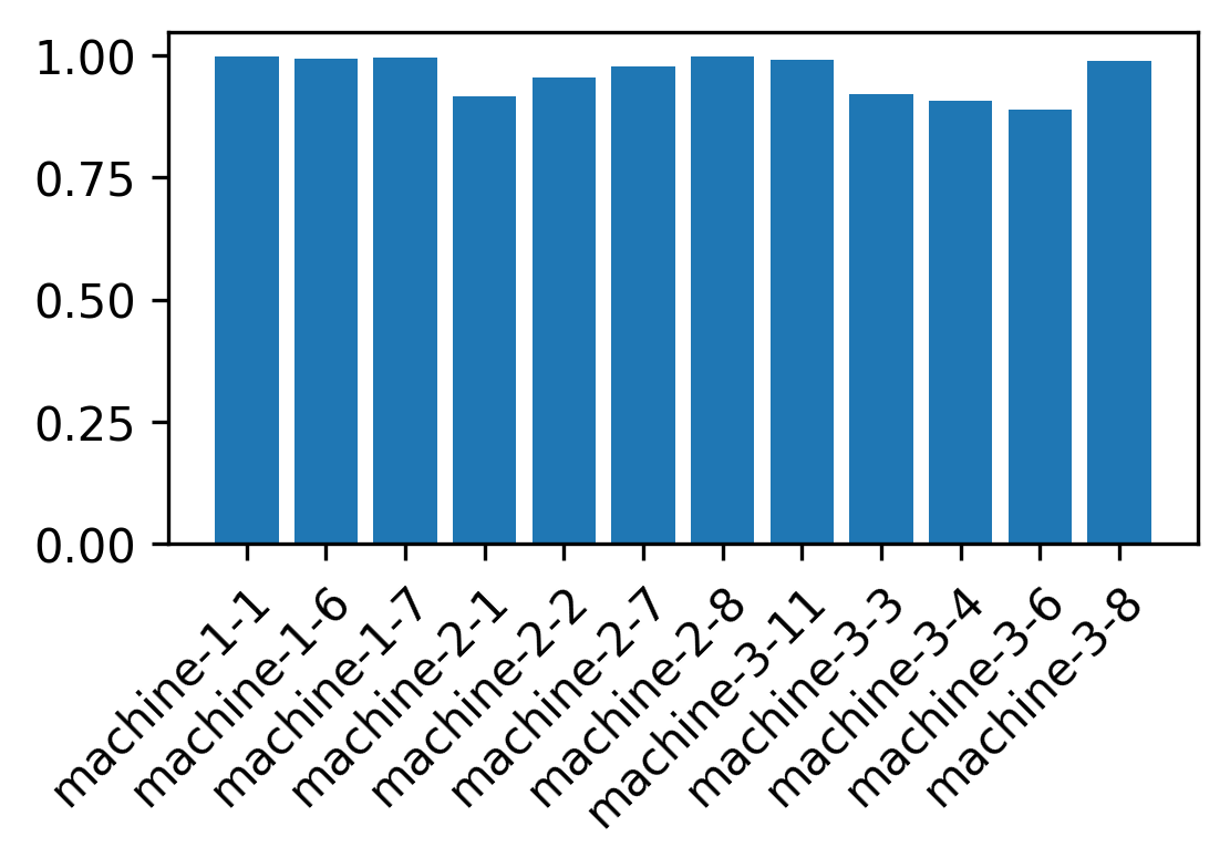
After assessing the performance on the test set, we obtain an F1 score above 0.95 for most of the machines in the dataset. Due to different methodologies we can’t do a fair comparison with scientific works on the same dataset, but that’s a satisfying result! Detailed results for each machine are shown in the bar chart below:
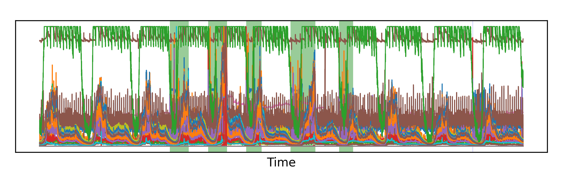
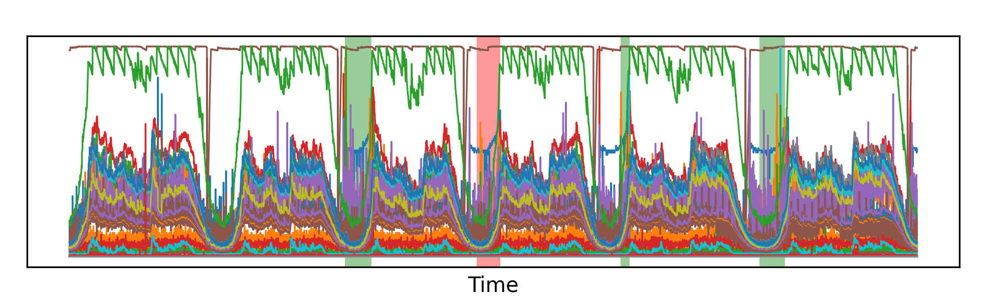
What can be interesting is to actually go and take a look at what the model is classifying. In the picture below, I show a section of the test set for two different machines, and I highlight the areas that have been correctly identified as anomalies, as well as any false negatives or false positives. What’s immediately striking is that identifying the anomalies with the naked eye appears to be an extremely hard task; however, the models seem to do just fine in most circumstances. In fact, the few errors that the model makes are often false negatives (the model didn’t notice an anomaly). False positives (anomalies being reported when in reality there is none) appear to be rare.
That’s our anomaly detection system.
Conclusion
There are multiple types of anomaly detection problems: in this article, we built a neural network model for anomaly detection on sequential data (time series). While we used relatively basic techniques to build our model, the same framework is applicable to numerous problems of similar nature.
Let me end with a word of caution: even if the code itself can look simple, there are nuances that one should keep in mind when building any machine learning system, such as data splitting, normalization, and a proper model selection. Make sure you fully understand these concepts before deploying a model, or your system – even if it performs well on paper – may not be able to generalize when deployed in the real world.
References
-
Rumelhart, David E., Geoffrey E. Hinton, and Ronald J. Williams. “Learning representations by back-propagating errors.” Nature, 323, 533–536. 1986. ↩
-
Pascanu, Razvan, Tomas Mikolov, and Yoshua Bengio. “On the difficulty of training recurrent neural networks.” International conference on machine learning. Pmlr, 2013. ↩
-
Cho, Kyunghyun, et al. “Learning Phrase Representations using RNN Encoder–Decoder for Statistical Machine Translation.” Proceedings of the 2014 Conference on Empirical Methods in Natural Language Processing (EMNLP), pages 1724–1734, Doha, Qatar. Association for Computational Linguistics. 2014. ↩
-
Hundman, Kyle, et al. “Detecting spacecraft anomalies using lstms and nonparametric dynamic thresholding.” Proceedings of the 24th ACM SIGKDD international conference on knowledge discovery & data mining. 2018. ↩ ↩2
-
Su, Ya, et al. “Robust anomaly detection for multivariate time series through stochastic recurrent neural network.” Proceedings of the 25th ACM SIGKDD international conference on knowledge discovery & data mining. 2019. ↩
-
Li, Zhihan, et al. “Multivariate time series anomaly detection and interpretation using hierarchical inter-metric and temporal embedding.” Proceedings of the 27th ACM SIGKDD conference on knowledge discovery & data mining. 2021. ↩